Build

Now I have received 2W metal film resistors from Mouser, and I have built the plate capacitor solution with a piece of circuit board material that is held in place with nylon bolts. This is mechanically quite secure:

Picture of inside of tap

Measuring with NanoVNA Saver

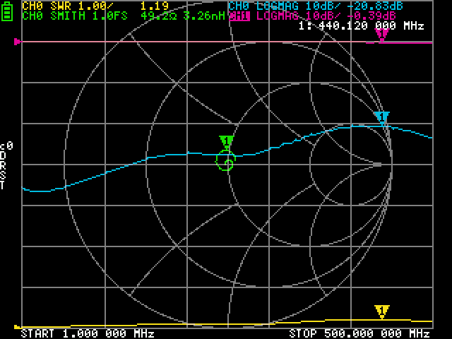
I figured out how to connect the nanoVNA to the computer with NanoVNA Saver. This allows me to either save a screenshot of what I saw while watchin the tiny screen when I adjusted the length of the small wire capacitor that is parallel to the power resistors:

NanoVNA screenshot

This shows that the power tap works quite well from 1 to 500 MHz, minimum return loss is almost 21 dB, at 440 MHz. The through insertion loss is very small.

Attempts to load NanoVNA touchstone files into R

There is a package by Aaron Anderson, rftk: RF Toolkit that supposedly can read touchstone files, do RF calculations and display data using ggplot.

library(tidyverse)
library(rftk)

Now, it should be possible to read the touchstone files saved by NanoVNA saver:

df_thru <- read_snp("40dB_pad.s2p")
df_pad <- read_snp("40dB_pad_attenuation.s2p")

We can take a look at the content of one of these files:

head(df_thru)

## # A tibble: 6 x 4
##   parameter frequency        db     ang
##   <chr>         <dbl>     <dbl>   <dbl>
## 1 S11         1000000  -35.5    177.   
## 2 S21         1000000   -0.0802  -0.204
## 3 S12         1000000 -Inf        0    
## 4 S22         1000000 -Inf        0    
## 5 S11         5990000  -36.1    171.   
## 6 S21         5990000   -0.0834  -1.15

The S12 and S22 parameters are not available in from the Nano VNA.

So we can now plot the return loss and insertion loss of a through connection:

Similarly, I have another set of measurement, with the VNA from input to the attenuated tap (and 50 ohm termination of output).

In theory, it should also be possible to plot these data on a Smith chart, there is a geom_smith extension to ggplot. The required aesthetics to the geom_smith are freq, smag, and sang. Frequency must be in Hz. From the example in the help, it is clear that sang is angle in radians (whereas the file was read with angles in degrees). I suspect that the smag might be the magnitude of the reflection coefficient, in which case \[|\Gamma| = 10^{S_{11}/20},\] with \(|\Gamma|\) being the magnitude of the reflection coefficient. Let’s try to put that into the Smith chart command.

And for the attenuation output:

I suspect that there are commands in rftk to do the conversion between S-parameters and reflection coefficient, but it seems as if the documentation is still not finished.